The Size of LLMs Explained and the Key Role of Quantization

A version of this article was initially published in French on 3 June 2025. on dev.to: link

0 – Introduction

Large Language Models (LLMs) raise a central question: why are they so massive in size, and why do they require such high computing power?

LLMs are trained on vast amounts of diverse text. They learn to detect patterns, understand relationships between words, and grasp nuances, which enables them to generate text on various topics, even those not covered during their training. This ability to generate text, even on new subjects, relies on a key element of LLMs: their parameters.

These parameters are numbers (usually floating-point numbers) that are gradually updated during training. Initially they are set randomly, then they get optimized through learning algorithms and subsequent phases such as fine-tuning, until they form a capable model. The number of these parameters determines directly the size of the LLM.

Even the smallest language models, like Llama 3.2 1b, have one billion parameters. As for the largest ones, like GPT-5, they are estimated to have over a trillion parameters. But why is such a huge number of parameters necessary? The answer lies in their representation as numerical values: encoding the subtleties of human language requires millions, even billions of precisely calibrated values. This complexity explains the technical challenges that LLMs pose in terms of memory and computation, and justifies the use of techniques like quantization, which aim to reduce their footprint while preserving their performance.

We will explore throughout this article how this architecture leads to considerable sizes, what technical challenges it raises, and how quantization can help make these models more accessible.

---

1 – How Computers Represent Data

Computers are machines that use electricity to function and store data. But how is this possible? In simple terms, we can say that a circuit carries an electric current or not. We can therefore represent its state with a 1 (with current) or a 0 (no current). By combining a large number of these circuits, we obtain a system capable of manipulating sequences of 0s and 1s, called bits, to represent any information.

However, in order for this system to work coherently and in order for computers to understand each other, it is essential to define shared conventions. This is why standards like ASCII, UTF-8, and IEEE 754 were created. They allow each sequence of bits to be associated with a precise meaning. For example, according to the ASCII standard, the letter k is encoded by the binary sequence 01101011.

The IEEE 754 standard is used to represent floating-point numbers in binary, to ensure precise and consistent calculations between different computer systems. It defines several representation formats, notably half-precision (16 bits), single precision (32 bits), and double precision (64 bits).

For example, a single-precision number uses 32 bits, that is 32 binary digits (0 or 1), while a half-precision number only uses 16. Since 8 bits make up a byte which is the fundamental unit of computer storage, a 16-bit floating-point number takes 2 bytes, and a 32-bit floating-point number takes 4 bytes. This means that each floating-point value stored in memory or on disk takes up a specific amount of space that is directly linked to its precision: the higher the precision, the more space is required.

---

2 – The Approximate Nature of Decimal Representation

Floating-point numbers pose a particular challenge because computers have to represent them in binary within a limited storage space. This means that seemingly simple numbers, like 0.1 or 0.2, cannot be represented with exact precision. They are therefore stored as approximations, which introduces small round-off errors. While individually insignificant, these errors can accumulate over successive calculations and affect the precision of results.

Why this approximation? Let’s take a constant like π (Pi) whose decimal expansion is infinite. So, how to represent it with perfect precision? It’s impossible: being irrational, π cannot be expressed exactly with a finite number of digits. Conversely, integers, however large they may be, represent finite and exact values as long as enough bits are allocated to them. For example, storing the diameter of the solar system in millimeters would only require about 54 bits. With floating-point numbers, on the other hand, we it’s a different story: although values like π are small in magnitude, their binary representation in binary format always requires an approximation. The more digits we want to capture, the more memory must be allocated. This is the fundamental trade-off: while an integer can be represented exactly, floating-point numbers can only approximate reality, even with high-precision formats. In other words, any representation of an irrational number like π is, by nature, an approximation, and the round-off error it introduces never disappears completely.

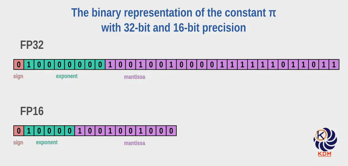
To illustrate this approximation phenomenon, let’s take π up to the 40th decimal:

3.1415926535897932384626433832795028841971

If we want to store it on a computer, the precision of the representation will depend on the allocated memory space:

16-bit space:

Binary representation	0100001001001000
Stored value	3.140625
Error	0.0009676535897932384626433832795028841971

32-bit space:

Binary representation	01000000010010010000111111011011
Stored value	3.1415927410125732421875
Error	-0.0000000874227800037248566167204971158029

The error value indicates the difference between the real value of π (up to the 40th decimal) and its approximations in the 16-bit and 32-bit formats. Although both errors are relatively small and often negligible, the 16-bit error is about 10 times larger than that in 32 bits. In fields like machine learning, an increase in error by a factor of 10 can have a significant impact on model performance. Thus, 32-bit formats are preferred for parameters requiring high precision. 16-bit formats remain used for less sensitive parameters, notably in the context of mixed-precision training, which allows reducing model size and accelerating training while maintaining high performance.

It should be noted that this difficulty of representing floating-point numbers in binary is not limited to irrational numbers, but also extends to certain rational numbers, including those with a finite decimal expansion. Here is how the number 0.1, which has a unique decimal expansion, is stored:

16-bit space:

Binary representation	0010111001100110
Stored value	0.0999755859375
Error	0.0000244140625

32-bit space:

Binary representation	00111101110011001100110011001101
Stored value	0.100000001490116119384765625
Error	-0.000000001490116119384765625

This floating-point number approximation phenomenon can be observed in many modern programming languages like Python or JavaScript. For example, adding 0.1 to 0.2 can be surprising: instead of getting 0.3, the result is often 0.30000000000000004. This illustrates the limits of binary representation imposed by the IEEE 754 standard.

# Python
a = 0.1
b = 0.2
print(a + b) # output: 0.30000000000000004

// Javascript
const a = 0.1;
const b = 0.2;
console.log(a + b); // output: 0.30000000000000004

---

3 – Impact on LLM Size

We have demonstrated that LLMs are enormous collections of floating-point numbers. But why not integers?

3.1 – Why Use Floating-Point Numbers Instead of Integers for LLM Parameters?

One might wonder, given their imprecision, why LLMs use floating-point numbers instead of integers. The answer lies in the fine-grained precision and wide range of values needed to represent the parameters of these models. Integers, although exact, are poorly suited to express the tiny variations and vast dynamic range necessary for neural calculations. Even if we can store a very large value, like the diameter of the solar system in millimeters with only 54 bits, this is not enough to capture subtle differences between weights and activations in a neural network.

Floating-point numbers, on the other hand, make it possible to efficiently represent both very large and very small values in a compact format, which is essential for modeling the linguistic nuances that LLMs learn. Furthermore, modern GPUs (graphics processing units) and NPUs (neural processing units) are optimized for this type of arithmetic, making operations not only possible, but also fast and efficient. Despite their approximation, floating-point numbers remain the most suitable solution to train LLMs.

3.2 – So, What Bit Precision for the Parameters?

Training LLMs requires billions of mathematical operations across extremely large neural networks. In this context, numerical precision is essential: small errors can accumulate and compromise the stability or performance of the model. High‑precision formats like FP32 (32‑bit floating‑point) remain crucial for numerically sensitive components of training, such as maintaining master weights, storing optimizer states, and performing certain reductions or normalization operations.

Modern training, however, increasingly relies on lower‑precision formats like FP16 or BF16 to accelerate computation and reduce memory usage. These formats are used for most forward and backward operations, including gradient calculations. Yet, because FP16 has limited dynamic range, it can introduce numerical instability if used for all parts of training. For this reason, frameworks employ mixed‑precision training, where FP16 is used for bulk tensor operations, while FP32 is retained for critical steps like weight updates and optimizer calculations.

In summary, the greater the numerical precision and dynamic range of a format—its ability to represent values across many orders of magnitude—the better a model can capture subtle patterns in the data. This expressive capacity makes high‑precision arithmetic a foundational component of effective LLM training.

3.3 – Impact on LLM Size

To fully understand the extent of memory requirements, let’s take a simple example: with 32-bit precision, each parameter takes 4 bytes. A model with 7 billion parameters, which is considered relatively small, requires:

32 bits = 4 bytes
7,000,000,000 × 4 = 28,000,000,000 bytes
28,000,000,000 bytes = 28 gigabytes

This means that 28 GB of memory is needed just to store the model, not counting the additional resources needed for to run it. At this point, you might think: "No problem, I have a powerful machine with 128 GB of RAM and a high-end CPU. I can run it without any issues, right?" Well, not too fast, the following might make you reconsider your position.

4 – What Hardware for LLMs

The CPU (central processing unit) and the GPU (graphics processing unit) are optimized for fundamentally different tasks. A CPU is a general-purpose processor with a small number of powerful cores. It excels in sequential tasks, branching logic, and managing a wide variety of operations. A GPU on the other hand, is designed for parallelism, and contains thousands of smaller and simpler cores optimized to simultaneously perform many similar operations.

The CPU is like a craft workshop where a few highly skilled artisans work. These experts know how to execute varied and complex tasks, but their limited number makes them more suited to precise and sequential operations. The GPU, in contrast, resembles an ultra-optimized factory employing thousands of specialized workers. Each of them performs a simple and repetitive task, but their strength lies in their ability to act in parallel, allowing the factory to carry out millions of operations simultaneously.

Similarly, system RAM and VRAM (Video RAM, or GPU memory) are fundamentally different. System RAM is slower and optimized for flexibility and capacity, while VRAM is designed for speed and high-bandwidth data throughput, suitable for feeding the GPU cores without bottleneck. Modern system RAM (for example, DDR4 or DDR5) offers bandwidths of about 25 to 70 GB/s. On the other hand, high-end VRAM like GDDR6X or HBM2e can reach over 700 to 1000 GB/s. That’s more than an order of magnitude faster. This lightning speed is essential for the mathematical workload types used in running large language models.

This is why a GPU with only 16 GB of VRAM can cost more than a CPU and 128 GB of RAM combined, because it’s not just about capacity; it’s about the speed and structure of computation and data transfer. GPUs are specially designed to perform massive matrix multiplications, the basic mathematical operation in neural networks, at high speed and in parallel.

4.2 – How GPUs Excel at Running LLMs

Running LLMs is essentially enormous running stacks of matrix operations. Each token you enter must pass through layer after layer of arithmetic, involving billions of parameters. These calculations are massively parallelizable, meaning they can be performed simultaneously, and this is where GPUs excel.

Because GPUs are capable of executing thousands of these matrix operations in parallel, they significantly outperform CPUs in tasks like inference (using a trained model) and training (configuring the model’s weights). Not only that, but VRAM ensures that all the model’s parameters and intermediate data can sit right next to the computing cores, ready for instant access without needing to go through slower system buses.

4.3 – So Capacity Isn’t Everything

Even with 128 GB of RAM capable of loading a 28 GB model, your powerful computer is not designed to run it in real-time. The RAM is slower, the CPU has fewer parallel cores, and the memory bus does not allow sustained high-bandwidth access, as required by LLMs. Running a modern LLM on CPU is like running a modern video game with integrated graphics: it can work, but not in a usable manner. The problem is not memory capacity, but access speed and parallel processing. Even a CPU like Intel i9 with 24 cores remains limited compared to GPUs like the RTX 4090, equipped with over 16,000 specialized cores capable of executing thousands of threads simultaneously, much more efficient for matrix and tensor operations. Having a lot of RAM is therefore not enough: the real constraint is the ability to transfer and process data efficiently, which GPUs, with their high-bandwidth VRAM and massive parallelism, do very well. CUDA (Compute Unified Device Architecture), Nvidia’s computing platform, enables the execution of kernels on thousands of threads, fully exploiting GPU architecture for fast, low-latency processing.

It should be noted that Apple’s unified memory architecture in their recent machines equipped with SoC (system on a chip), allows the CPU and the GPU, which are integrated into a single chip, to share the same high-bandwidth memory (also integrated into the same chip), reducing transfer overheads and improving local LLM execution. Tests on these machines have demonstrated that they could easily run language models of certain sizes with low power consumption. However, most deep learning tools (PyTorch, TensorFlow) remain optimized for CUDA and its libraries like cuBLAS and TensorRT, designed to accelerate matrix calculations and inference on Nvidia GPUs. This gives them a clear advantage in performance and compatibility. Unified memory remains a promising avenue: if other manufacturers adopt it, local LLM inference could become more efficient and accessible on more personal machines.

4.4 – But Why The Parallelism? Can’t We Do Otherwise?

Since the publication of Google’s landmark paper "Attention Is All You Need" in 2017, machine learning has undergone a major revolution with the introduction of the Transformer architecture. Unlike previous sequential models, Transformers allow for the simultaneous processing of all tokens in a sequence, thanks to the multi-head attention mechanism—eliminating the need for sequential processing.

Modern language models are based on this architecture. When a user enters a prompt, each token is converted into a vector and processed in parallel across the different layers of the model. This parallel processing is essential to effectively capture contextual relationships between tokens.

This approach requires significant parallel computing capability, which GPUs naturally offer as we have demonstrated. In summary, the parallelism intrinsic to Transformers makes the use of GPUs essential for LLM training and inference, in order to effectively manage the computational and memory loads associated with large prompts.

4.5 – Summary

unning large language models locally requires specialized, expensive hardware—such as powerful GPUs with high-bandwidth memory and massively parallel architectures. This reality may seem discouraging, but before frustration sets in, know that solutions exist to circumvent these limitations. Certain approaches make it possible to efficiently run LLMs on much more modest hardware.

---

5 – Quantization

5.1 – Definition

Quantization is a process of representing numerical data with reduced precision to decrease its size or simplify its processing. It relies on replacing values from a large range of possible levels with approximations using a more restricted set. This reduction in precision limits storage, bandwidth, and computing power requirements, at the cost of a generally accepted loss of information.

5.1.1 – Examples to Simplify the Concept

5.1.1.1 – Reducing Bit-Rate in Audio Files

We can apply quantization to an audio file by reducing its bit-rate, which is the number of kilobits per second (kb/s) used to encode the sound. For example, an audio file encoded at 320 kb/s offers quality very close to the original, but requires more storage space. By reducing this bit-rate to 128 kb/s or even 64 kb/s, the file size decreases considerably, at the cost of a loss of detail in the sound. The level of compression depends on the intended use. For a piece of classical music, where nuances and the richness of instruments are important, a high bit-rate (like 256 or 320 kb/s) is preferable to preserve listening quality. For an audiobook of a novel, a lower bit-rate (64 or 96 kb/s) is often sufficient, because the main objective is to transmit the voice in a clear and intelligible manner, even if some sonic details are lost.

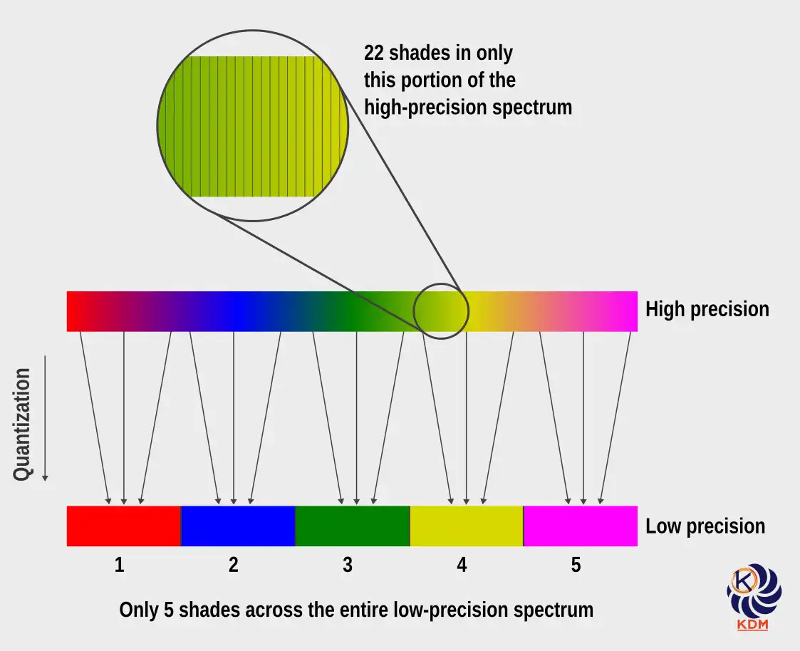
5.1.1.2 – Color Quantization in Images: A Compression Technique

In digital image processing, quantization involves reducing a continuous spectrum of colors to a more restricted palette. This simplification enables data compression by using a limited number of colors, which reduces file sizes and computational requirements. Although this operation involves some loss of information, it is generally designed to preserve the overall visual appearance of the image, making the compression effective without significantly altering perceived quality.

5.1.2 – Analogy: The Color Ball Sorting Challenge

Imagine you have a huge pile of small balls, each a different color—not just different colors, but also different shades, from the darkest to the lightest tones. Your challenge? Sort the balls by color into separate boxes. Once sorted, you must send the boxes to a person who will evaluate your sorting skills. Sounds fun, doesn’t it? Well, there’s a catch: you have a limited budget for both buying boxes and transportation. This means you will have to make choices.

• If you want the highest possible score, your sorting must be super precise. This means using a separate box for each shade. But then, you will end up with many boxes, and that means you will need a big expensive truck to move them. When you check your budget, it’s clear: it’s not enough.

• So you start thinking smarter. What if you grouped similar shades together? Fewer boxes mean lower costs, and you won’t need a huge truck. Admittedly, the sorting won’t be perfect, but it could be good enough to impress the person who will judge your performance while staying within budget limits.

• In the end, you find a middle ground. You buy just enough boxes to keep things organized without overdoing it. You sort by grouping similar shades into the same box and prepare everything for transport in a truck at a price that doesn’t exceed your budget.

5.2 – LLM Quantization

Model quantization is a technique that intentionally reduces the precision of numerical representations, from 32-bit floats to 16 bits or even 8 bits. This process significantly decreases model size, accelerates calculations, and reduces energy consumption—benefits that are crucial for deployment on edge devices or in environments where efficiency is paramount. However, reducing the number of bits means that each parameter is represented with less precision, which can subtly affect the arithmetic operations that underlie model performance. It is therefore essential to find a balance: the model must retain sufficient precision to generate quality content, while benefiting from memory efficiency and speed. Advances like quantization-aware training (QAT) help mitigate performance losses, ensuring that these compact models remain effective and reliable after quantization.

5.3 – Preparation for Quantization with QAT

Certain techniques are employed during LLM training to prepare the model for future low-precision Quantization. One of the most effective techniques is quantization-aware training (QAT), which introduces artificial quantization steps to simulate the behaviour of low-precision arithmetic. These steps reproduce the rounding, clipping and noise effects inherent in reduced formats without altering the stored values: the weights remain in high precision (for example, 32 bits).

Through this training under simulated constraints, the model learns to become robust to the perturbations it will encounter during deployment. Once training is complete, the simulated Quantization operations are replaced with real Quantization, and the weights and activations are converted to formats such as FP16 or INT8 (an 8-bit integer), using calibrated scale factors and zero points. Additional optimisations, such as fusing the batch normalisation with previous layers, further enhance efficiency. The result is a quantized model that is lighter and faster yet retains a level of precision close to that of the original full-precision model.

5.4 – Good Results with FP4, Really?

Research on quantization is progressing rapidly, paving the way for faster, more compact, and less energy-intensive models. A landmark paper published in early 2025, "Optimizing Large Language Model Training Using FP4 Quantization" proposes a bold advance: training LLMs using a precision of only 4-bit floating-point (FP4). This format is not even defined by the IEEE 754 standard, which underscores how much this approach breaks from the 16-bit or 32-bit formats traditionally used.

What Makes FP4 Special

FP4 adopts a fundamentally different approach to quantization compared to integer-based formats such as INT8 or INT4, which rely on fixed-point arithmetic with uniformly spaced representable values. Instead, FP4 preserves a floating-point structure within an extremely compact 4-bit representation (typically an E2M1-style format, depending on hardware implementation). This allows it to retain a limited but useful dynamic range, enabling the representation of both very small and relatively large values despite the extreme reduction in precision.

However, operating at such low precision introduces significant numerical stability challenges. To address these limitations, modern FP4-enabled systems rely on a combination of complementary techniques:

1. Block-wise dynamic scaling: Rather than applying a single global scale factor, weights are quantized in small blocks, each with its own scaling parameters. This improves local fidelity by preserving relative structure within weight groups.

2. Strategic mixed precision: Numerically sensitive operations—such as normalization layers, accumulations, or certain activation pathways—are executed in higher precision formats (e.g., FP8 or FP16), ensuring stability while maintaining the benefits of FP4 for the majority of tensor operations.

3. Stochastic rounding: In some training-aware or simulation contexts, quantization may incorporate probabilistic rounding rather than deterministic nearest-value mapping. This reduces systematic bias introduced by repeated low-precision rounding, improving long-term convergence behavior.

Together, these techniques allow FP4-based systems to achieve substantial gains in memory efficiency and throughput, while mitigating the inherent limitations of ultra-low precision arithmetic.

Additional adjustments include clipping (trimming) extreme values and smoothing calculations during training. The result is that despite a drastic reduction in floating-point precision, models quantized in FP4 show minimal performance degradation on major benchmarks compared to models trained with full-precision.

It should be noted, In earlier work, many results on FP4 precision were obtained in simulated environments, raising questions about their practical impact. Since then, this landscape has changed significantly. Native FP4 computation is now supported in hardware, most notably through Nvidia’s Blackwell architecture and its associated TensorRT ecosystem, including the GeForce RTX 50 series GPUs. As a result, the speed and energy efficiency gains of FP4 are no longer purely theoretical: they can now be observed in real-world inference workloads, particularly in large-scale AI systems. This marks a concrete turning point, as ultra-low-precision formats like FP4 transition from experimental research concepts to practical tools driving a new generation of AI-optimized hardware.

5.5 – Ultra-Low Precision Quantization: Toward Practical LLM Inference at Scale

While floating-point formats such as FP16 and FP32 have long dominated language model (LLM) training, a new generation of ultra-low precision quantization techniques is reshaping inference. These approaches go beyond standard 8-bit integers, achieving effective compression levels as low as ~1.5 to 3 bits per weight through a combination of grouping, mixed-precision encoding, and entropy-aware representations.

Rather than introducing new native numeric formats, these methods map continuous model weights into compact discrete representations, significantly reducing memory usage. For instance, experimental work on models such as DeepSeek-R1-671B has demonstrated substantial compression—from hundreds of gigabytes in FP16 down to well below 200 GB—using advanced dynamic quantization pipelines. While such results depend heavily on implementation details, they highlight the considerable redundancy present in large-scale models.

The primary benefit of ultra-low precision is not only reduced arithmetic complexity, but more importantly improved memory bandwidth efficiency and cache utilization—two critical bottlenecks in modern AI inference. Even when some numerical precision is lost, the overparameterized nature of LLMs often allows them to retain strong performance, yielding an effective trade-off between model size, speed, and accuracy.

Today, tools and ecosystems such as GGUF (used with llama.cpp), AWQ, GPTQ, and production frameworks like TensorRT increasingly automate these optimizations. Combined with modern GPUs and specialized accelerators, they enable the deployment of increasingly capable models on consumer-grade hardware, including laptops and edge devices.

Ultra-low precision quantization is therefore not merely a theoretical optimization, but a key enabler of efficient, scalable, and accessible AI systems.

---

6 – Conclusion: The Future of Local LLMs Looks Increasingly Real

As language models continue to grow in size and capability, quantization techniques are becoming essential to making them widely accessible. Advances in ultra-compact representations—alongside hardware support for formats such as FP4 and increasingly specialized inference architectures—are accelerating a shift toward more efficient deployment.

This evolution makes it increasingly feasible to run capable language models locally on personal devices, particularly in compressed or task-specific forms. Such a transition offers tangible benefits: improved privacy, reduced latency, and greater control over data and personalization.

While large frontier models still require substantial infrastructure, the gap is narrowing. Continued progress in quantization, model architecture, and hardware-software co-design suggests a near future where high-quality AI systems will be not only more efficient, but also more widely and directly accessible.